“Statistics is not perfect, but it is beautiful and exquisite! ”

Theoretical Derivation

This post is heavily focused on the mathematical proof and theoretical derivation, which doesn’t be discussed much in the “Statistics” Post.

Will be an appendix of it.

Gaussian Distribution

Normally, we have Gaussian Distribution: $X\sim \mathcal{N}(\mu ,{\sigma }^2)$$X\sim\mathcal{N}(\mu, \sigma^2)$.

We can now have $(X-\mu )\sim \mathcal{N}(0,{\sigma }^2)$$(X-\mu)\sim\mathcal{N}(0, \sigma^2)$, which is symmetric odd-function.

As for the properties of PDF and CDF, we have:

Gaussian Probability Tables and Quantiles

Means of Gaussians

For $\mathbb{E}[x]=\mu$$\mathbb E[x] = \mu$,

For $\mathbb{E}[x^2]={\sigma }^2+{\mu }^2$$\mathbb E[x^2] = \sigma^2 +\mu^2$,

For $\mathbb{E}[x^3]=3\mu {\sigma }^2+{\mu }^3$$\mathbb E[x^3] = 3\mu\sigma^2 +\mu^3$,

Patch up $x^3$$x^3$ into $(x-\mu {)}^3$$(x-\mu)^3$,

So we have, substitutes with $\mathbb{E}[x^2]$$\mathbb E[x^2]$ and $\mathbb{E}[x]$$\mathbb E[x]$ formulas:

For $\mathbb{E}[x^4]=3{\sigma }^4+6{\mu }^2{\sigma }^2+{\mu }^4$$\mathbb E[x^4] = 3\sigma^4 +6\mu^2\sigma^2 + \mu^4$,

Patch up $x^4$$x^4$,

So we have,

For $\mathbb{E}[{\overline{X}}_n]=\mathbb{E}[X_1]$$\mathbb E[\bar{X}_{n}] = \mathbb{E}[X_{1}]$,

For $\mathbb{E}[XY]$$\mathbb E[XY]$,

The expectation of the product of X and Y is the product of the individual expectations: E(XY ) = E(X)E(Y ).

Variance of Gaussians

For $\mathbb{V}[x]={\sigma }^2$$\mathbb V[x] = \sigma^2$,

With integral formulas step by step, we can get:

Which can be simplified with expectation substitutions we concluded above:

For $\mathbb{V}[x^2]=2{\sigma }^4+4{\sigma }^2{\mu }^2$$\mathbb V[x^2] = 2\sigma^4+4\sigma^2\mu^2$,

$V({\overline{X}}_n)=\frac{{\sigma }^2}{n}$$V(\bar X_n)=\large\frac{\sigma^2}{n}$

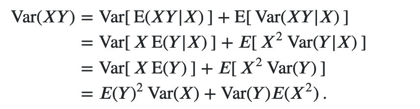
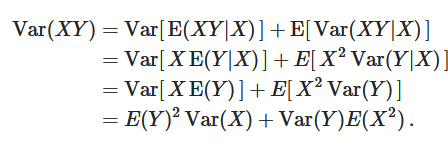
Var(XY)

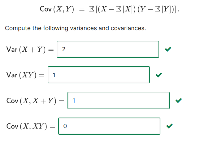
Covariance

Normally, we have standard covariance formula between variable $x$$x$ and $y$$y$,

pdf

You should have something like:

Now:

So:

Covariance of Gaussians

Recall that the covariance of two random variables $X$$X$ and $Y$$Y$ denoted by $\text{Cov}(X,Y)$$\text{Cov} (X,Y)$ is defined as:

Var[X+Y] = Var[X] + Var[Y] + 2∙Cov[X,Y]

If the covariance between two random variables is 0, then they are independent?

False, the criterion for independence is $F(x,y)=F_X(x)F_Y(y)$$F(x,y)=F_X(x)F_Y(y)$

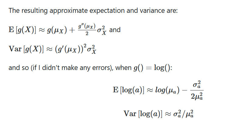
variance of ln function

Var[X] is known, how to calculate Var[$\frac{1}{x}$$\frac{1}{x}$]:

Using Delta Method,

You can use Taylor series to get an approximation of the low order moments of a transformed random variable. If the distribution is fairly 'tight' around the mean (in a particular sense), the approximation can be pretty good.

SO

often only the first term is taken

In this case (assuming I didn't make a mistake), with $g(X)=\frac{1}{X},\mathrm{Var}\left[\frac{1}{X}\right]\approx \frac{1}{{\mu }^4}\mathrm{Var}(X)$$g(X)=\frac{1}{X}, \operatorname{Var}\left[\frac{1}{X}\right] \approx \frac{1}{\mu^{4}} \operatorname{Var}(X)$.

The Property of Maximum

Given the IID r.v. $X\sim \text{Uni}(0,1)$$X\sim \text{Uni}(0,1)$, we have $M_n=max(x_1,\cdots ,x_n)$$M_n=\max(x_1,\cdots,x_n)$,

Then, because $X_n$$X_n$ are i.i.d. :

where$F_X(\cdot )$$F_X(\cdot)$ is the CDF of distribution.

Limitations

for anyconstant $c$$c$:

Food for thought:

What is the variance of the maximum of a sample?

Maximum of uniform random variables

$M_n$$M_n$

b = - (2*barX_n + 1.6448^2/n)

(2barX_n + 1.6448^2/n + sqrt((2barX_n + 1.6448^2/n) &2-4*barX_n^2) )/2

Mode of Convergence Examples

Example of a.s.

Let $U\sim \text{Uni}(0,1)$$U\sim \text{Uni}(0,1)$, $X_n=U+U^n$$X_n = U + U^n$ (raised to the power of $n$$n$)

Claim: $X_n\stackrel{\text{a.s}}{⟶}U$$X_n\overset{\text{a.s}} \longrightarrow U$

Proof:

With law of total probability, for any event $A$$A$,

So we have

Example 1 of $\mathbb{P}$$\mathbb P$ ,

Let $X_n\stackrel{iid}{\sim }Ber(\frac{1}{n})$$X_n \overset{iid}\sim Ber(\frac{1}{n})$ and $ϵ\in (0,1)$$\epsilon \in (0,1)$, we have

Example 2 of $\mathbb{P}$$\mathbb P$ ,

Let $U\sim \text{Uni}(0,1)$$U\sim \text{Uni}(0,1)$, $X_i=min{X}_i$$X_i = \min X_i$

Claim:$X_{(1)}\stackrel{p}{\to }O$$X_{(1)} \stackrel{p}{\rightarrow} O$,

Proof:

Fix $\epsilon >0$$\varepsilon>0$,

Example of complying $\mathbb{P}$$\mathbb P$ but not with a.s.

Let $U\sim \text{Uni}(0,1)$$U\sim \text{Uni}(0,1)$, $x$$x$ is more and more subdivided segmentation functions between [0, 1]:

Claim 1: $x_n\stackrel{p}{\to }U:\text{Fix}0<\epsilon <1$$x_{n} \stackrel{p}{\rightarrow} U: \text{Fix}\ 0<\varepsilon<1$

Claim 2: $x_n\bcancel{\stackrel{\text{a.s.}}{\to }}U$$x_{n} \enclose{downdiagonalstrike} {\stackrel{\text{a.s.}}{\rightarrow}} U$:

Quadratic equation