“Machine Learning, Deep Learning, Data Science, etc. are all in the same nexus – which is the bacically Probability plus Statistics. ”
Statistics, MIT 18.6501x
A useful book and a probability refer link.
Where will be covered:
Hoeffding's Inequality, Chebyshev Inequality
Asymptotic normality
Delta (
Mode of Convergence
Estimator
Probability Redux
Theorems and Tools
i.i.d. stands for independent and identically distributed .
r.v. denotes random variable
Law of Large Numbers (LLN)
According to the law, the average of the results obtained from performing the same experiment a large number of times should be close to the expectation value, and tend to be closer when n is even greater.
Let
Central Limit Theorem (CLT)
CLT establishes that when independent random variables summed up, their properly normalized sum tends toward a normal distribution even if the original variables themselves are not normally distributed,
where
Standard Gaussian means that this quantity will be a number between (-3, 3) with overwhelming probability, we have
Rule of thumb to apply CLT - normally, we require
Asymptotic normality
Assuming the sequence
Hence, the sample mean
Continuous Mapping Theorem (CMT)
CMT states that continuous functions preserve limits even if their arguments are sequences of random variables. A continuous function
It applies to
But how close is
Hoeffding's Inequality
What if
For bounded random variable, this is still Hoeffding’s Inequality we can say for any n.
Let
Here I need that my random variables are actfually almost surely bounded, which rules out like Gaussians and Exponential Random Variables.
How to choose
So let's parse this for a second… , if when
The square root of
So the conclusion is the average is a good replacement
Is this tight? That's the annoying thing about inequalities.
The above inequality could actually be e to the minus exponential of n (
Chebyshev Inequality & Markov Inequality
These two inequalities guarentees that upper bounds on
Markov inequality
For a random variable
Note that the Markov inequality is restricted to non-negative random variables.
Chebyshev inequality
For a random variable
Remark:
When Markov inequality is applied to
Triangle Inequality
Slutsky’s Theorem
Slutsky's Theorem will be our main tool for convergence in distribution.
Let
Then,
If in addition,
Delta (
https://en.wikipedia.org/wiki/Delta_method
Distribution
Discrete: Probability mass function
Bernoulli, Uniform, Binomial, Geometric
Gaussian Distribution
Notation:
Mean and Variance:
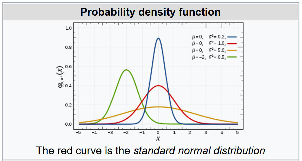
Probability Density Function:
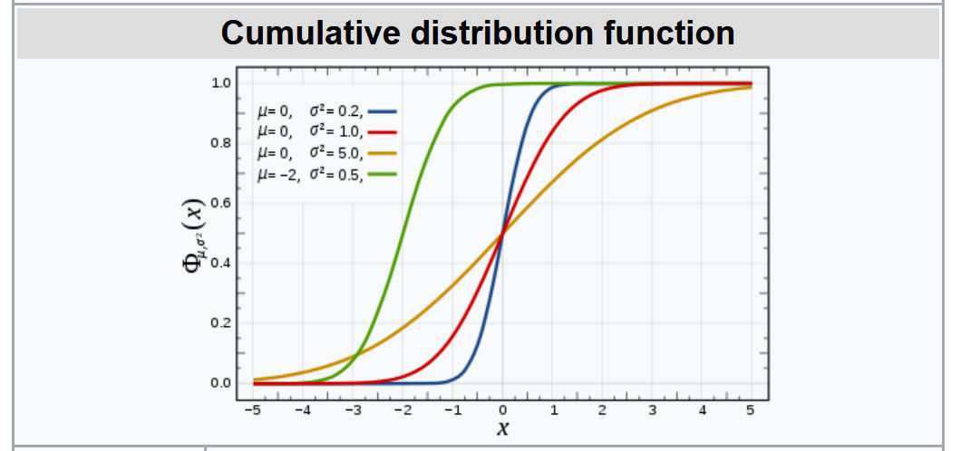
Cumulative Distribution Function:
Why we use Gaussian Distribution so frequently?
Normally, we use sample mean as our estimator. And the reason is because the Gaussian distribution is the thing that shows up as the limit of the CLT as the minute you start talking about averages.
Of the universe type of results, that says that if you take average of enough things, then it's going to go to a Gaussian.
The extreme value?
The value field of a Gaussian is
Yes, there exists extreme value, but they never really come into play. Because of the exponential can get really, really small. The Gaussian actually almost in a bounded interval.
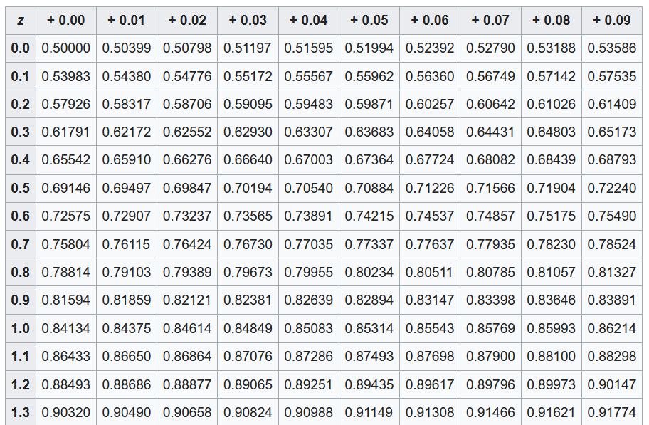
Gaussian Probability Tables
A Gaussian CDF (z-score) calculator.
Quantiles
| 2.5% | 5% | 10% | |
|---|---|---|---|
| 1.96 | 1.65 | 1.28 |
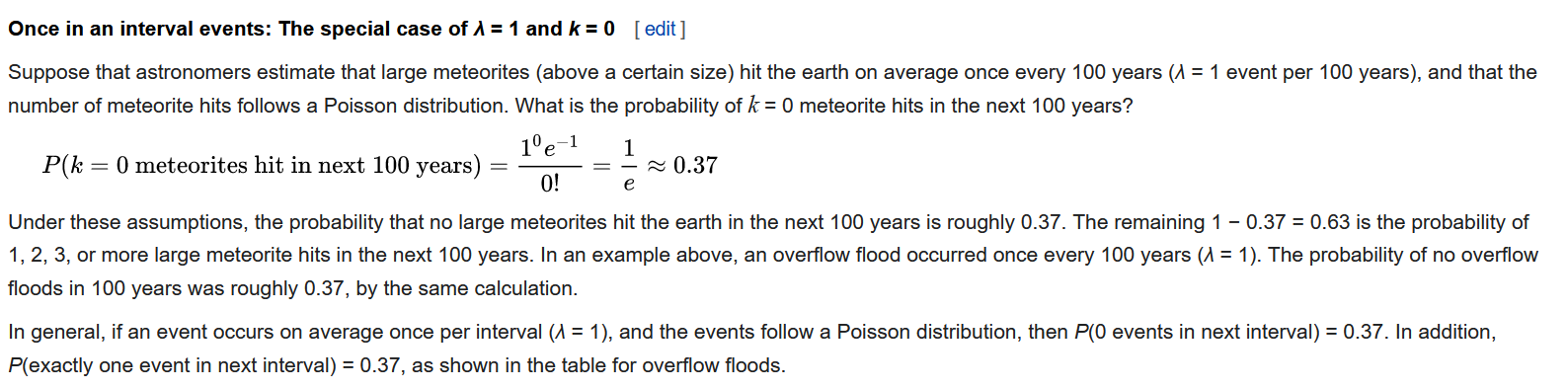
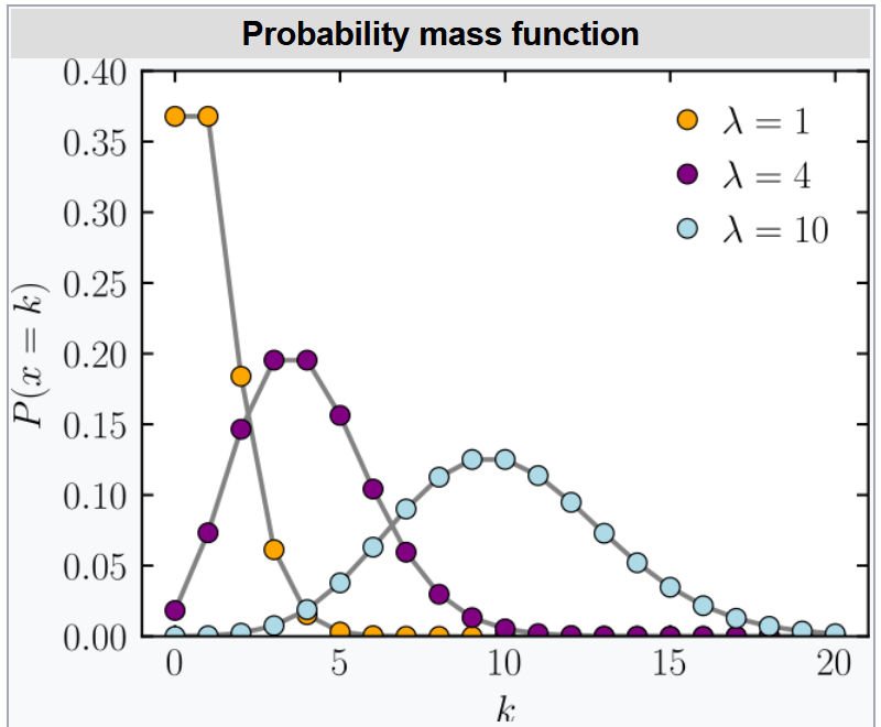
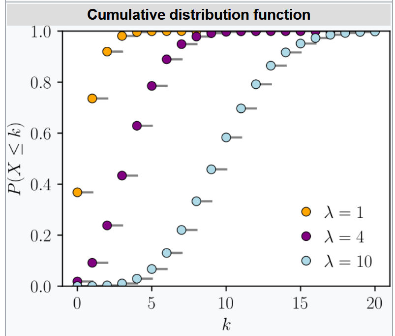
Poisson Distribution
The advantage of using poisson distribution is that n or p do not need to be known! This can make assumptions much easier.
Notation:
Mean and Variance:
Pre-require 0! = 1
Probability Mass Function:
Cumulative distribution function:
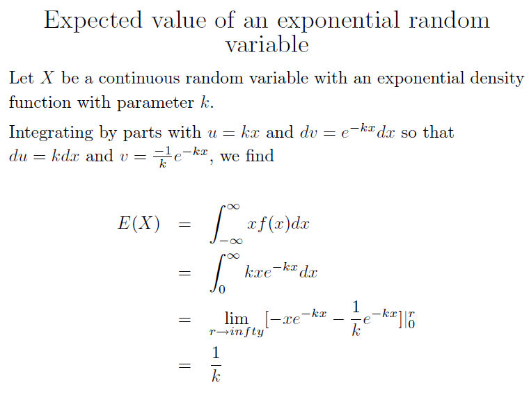
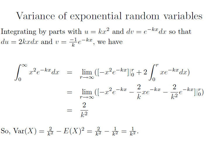
Exponential Distribution
sample space:
Mean and Variance:
Probability Mass Function:

Cumulative distribution function:

Gamma Distribution
Notation:
Parameters:
Mean and Variance:
Gamma Function:
Probability Mass Function:
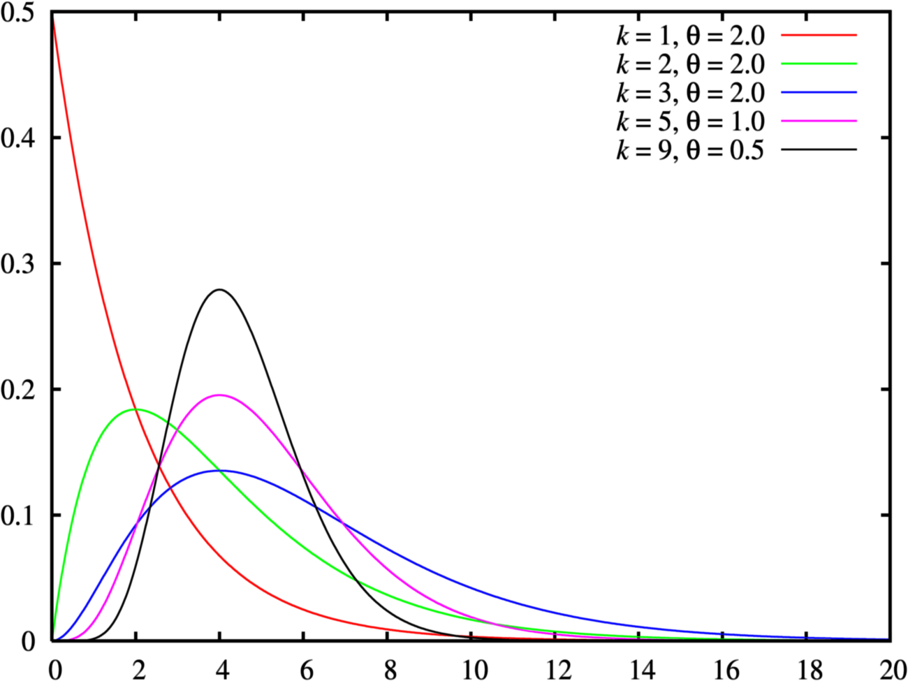
Cumulative distribution function:

Geometric Distribution
Such as : number of trials until a success
Geometric Distribution is either one of below two distribution:
The probability distribution of the number
The probability distribution of the number
Notation:
Mean and Variance:
Probability Mass Function:

Cumulative distribution function:


Binomial Distribution
Notation:
Mean and Variance:
Probability Mass Function:
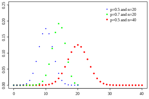
Cumulative Distribution Function:

In other words, there are a finite amount of events in a binomial distribution, but an infinite number in a normal distribution.
Bernoulli Distribution
Notation:
Mean and Variance:
PMF pmfs

Indicator Function
The indicator function of a subset
defined as
Derivative of indicator function
I have an indicator function
δ is symmetric. δ can be thought of as the derivative of the Heaviside function H(x)=1 for x>0, 0 for x<0.
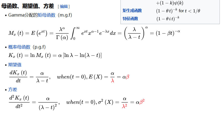
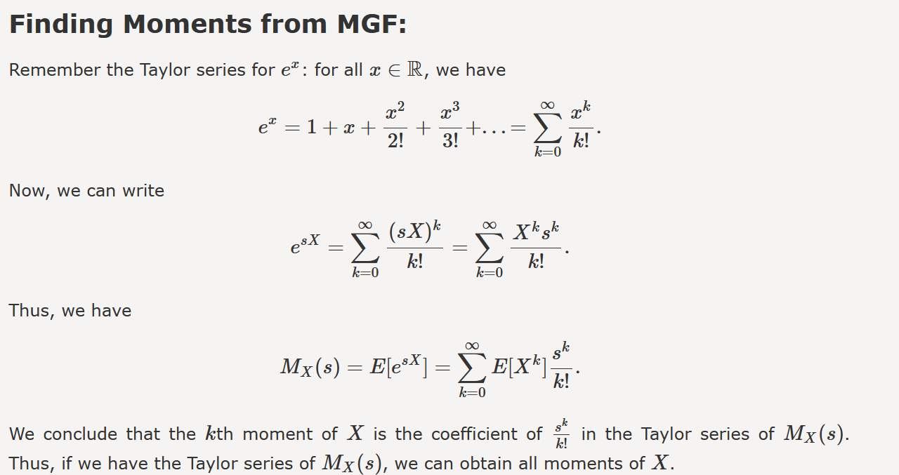
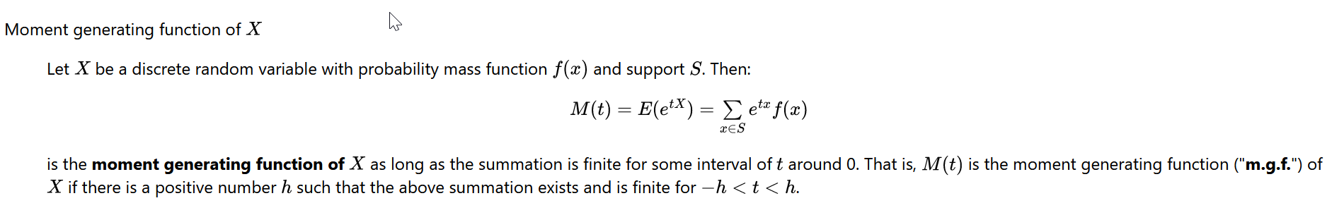
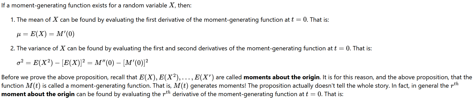
Moment Generation Function (MGF)
https://en.wikipedia.org/wiki/Moment-generating_function
expectation of moment generating function
https://online.stat.psu.edu/stat414/book/export/html/676
mixture distribution moment generating function
Useful…
Property of Distribution
We take Gaussian
Affine Transformation:
Standardization:
According to CLT, we assume
Symmetry:
Mode of Convergence
Three types of convergence, going from strong to weak.
Some examples are shown [here]
Almost surely (a.s.) convergence
So I created two sequences, and I want this to converge.
Convergence in probability
The probability that they depart from each other by something is going to be going to 0 as
Convergence in distribution
This just saying I'm going to measure something about this random variable, maybe it is distribution. For all continuous and bounded function
I'm just saying that its distribution is converging. My random variable is going to become the same as the probabilities for the second guy as
Properties
If
If
Convergence in distribution implies convergence of probabilities if the limit has a density (e.g. Gaussian):
Addition, Multiplication and Division Assume,
Then,
If in addition,
Warning: In general, these rules do not apply to convergence in distribution
Estimator
Normally, we have two estimator:
Compute the expectation of your random variable
Using Delta method
How can we decide how many samples (
Now we have our first estimator of
For
Our first estimator of
And averages of random variables are essentially controlled by two major tools: They are LLN and CLT.
What is the accuracy of this estimator?
What is the probability that
We don’t even know the trueandard and the observation
Modelling Assumptions:
Each r.v. and i.i.d
Measures of Distance
If we want to estimate mean of a Gaussian and we can compute the expectation, but not it doesn’t work for the the variance.
You can go into example and compute the variance, which is actually coming from the method of moments.
But it turns our we have a much more powerful method called the maximum likelihood method, but it is far non-trivial.